Introduction
The JRC Earth Observation Data and Processing Platform (JEODPP) is a versatile petabyte scale platform that serves the needs of a wide variety of projects [SBR+16][SBDM+17][SBDM+18]. This is achieved by providing a cluster environment for batch processing, a remote desktop access with a variety of software suites, and a web-based interactive visualisation and analysis ecosystem. These three layers are complementary and are all relying on data co-located with the processing nodes.
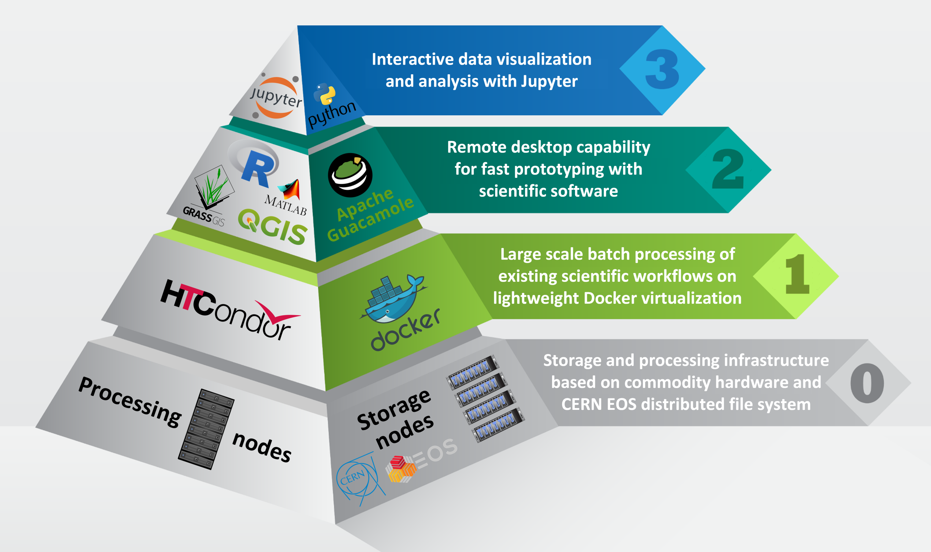
JEODPP infrastructure: synthetic view of the three service layers on top of the hardware layer [from [SBDM+17]]
This manual describes in detail, by providing both a tutorial section and a reference section, the upper component (the one labeled as 3 in the previous image): the Interactive data visualization and analysis based on Jupyter notebooks [DMBKS17].
An overview of the interactive processing operation mode integrated on the JEODPP is sketched in the following picture:
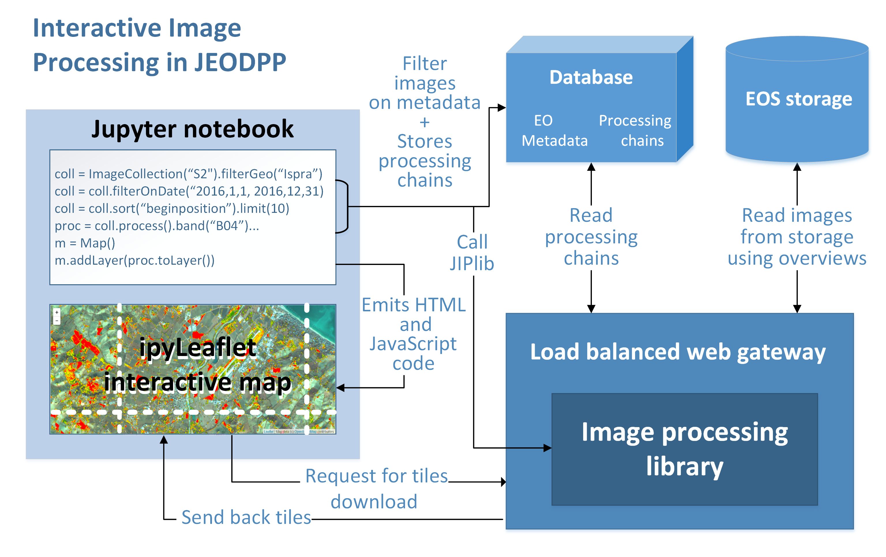
Interactive processing operation mode on the JEODPP
The Jupyter notebook provides a programming interface that can accommodate a variety of programming languages. The Python language was selected for its open source and its wide variety of packages for data scientists with processing, analysis, and visualisation capabilities. The Python code developed in the Jupyter notebooks is not directly executing the data processing. Indeed, the processing is merely defined as a deferred execution pattern that is only executed when needed. The code from the Jupyter notebook is translated into a JavaScript Object Notation (JSON) describing all processing and analysis logic that is matching the desired image processing chain object as well as the desired data on which it needs to be applied thanks to a selection process based on metadata information.
A key element of the Jupyter notebook is the interactive map display. This map relies on the Leaflet JavaScript mapping library, loaded into Jupyter notebook via the IPyleaflet extension [IPL]. The map contains a selectable base background layer for navigation. The deferred processing is executed when adding a processing chain as a display layer to the interactive map.
The OpenStreetMap [OSM] defines the default base map for the map viewer. Other base maps such as OpenTopoMap, OpenMapSurfer or the MODIS global composite of any specific date can be selected. Any given collection of images or vector layers can then be viewed on the top of the base maps while considering a user-defined opacity level. Available collections on the JEODPP platform are based on radar imagery (Sentinel-1), optical imagery (Sentinel-2, Landsat GLCF, MODIS, etc.), Digital Elevation Models (EUDEM, SRTM, etc.), as well as a series of raster layers such as the Global Human Settlement Layer and the Global Water Surface Layer. In addition, a user can easily create a new collection by importing his/her own data. Any raster collection can be combined with arbitrary vector data sets whether prede- fined or imported by the user. Examples of predefined vector datasets are: administrative boundaries (GAUL, NUTS, etc.), the Military Grid Reference System used for Sentinel-2 tiling, the Sentinel-2 relative orbits, and the European Natura 2000 protected areas.
The core components of the Jupyter-based interactive environment for geospatial data visualisation and analysis are schematised this figure:
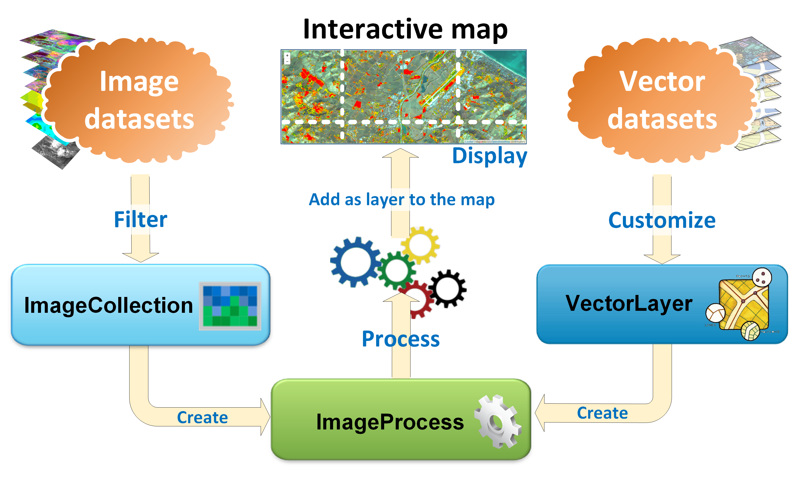
Raster and vector data in the JEODPP interactive visualisation and analysis [from [SBDM+18]]
The handling of raster and vector data, processing chains, as well as import/export capabilities are presented in the following three subsections.
Raster data management
The concept of image collection is inspired by the one proposed on the Google Earth Engine platform. Mote precisely, the JEODPP interactive library provides an ImageCollection class that allows users to search, select, and filter raster datasets based on a variety of criteria. Users can instantiate an ImageCollection from the relevant dataset (e.g., Sentinel-2 and Sentinel-1) and then choose a geographic location of interest to filter products that intersect a named location (based on calls to the GeoNames online service). Each metadata in the collection can then be used to refine the selection by using arithmetic, logical, and alphanumeric operators to get the set of images matching all search criteria. For example, all the images acquired in a specific time interval, which have a reduced cloud coverage and have been acquired by a specific sensor on a given relative or absolute orbit can be selected.
Vector data management
A section of the interactive library is dedicated to the management of vector datasets. Thanks to the mapnik library that allows vector to raster conversion based on rules, vector data are treated in the same way as raster data. The display of vector data can be easily customised by editing all visual attributes (colors, thicknesses, line and fill types, etc.) as well as constructing display legends based on data attributes (single or graduated col or legends) with colors selected from a vast palette library or directly specified by the user.
Data processing chains
From the instance of ImageCollection or VectorLayer, the user can generate a processing chain by applying data transformation operators to obtain the required analysis and visualisation result. Available operators include the following categories: pixel based operators (e.g., masking, filtering, and band arithmetic), index calculation (NDVI, NDWI, etc.), RGB combination (on-the- fly visualisation of three different processing chains in RGB mode), merging and blending (combination of two or more processing chains using alpha transparency), morphological operators, segmentation, legend management (using prede- fined legends or creating custom ones from a user-defined list of colors), etc. The resulting processing chain can then be added as a layer to the map and displayed inside the notebook with the ability to zoom and pan. The processing takes place on the basis of the user display requests: the displayed tiles are calculated in parallel and only at the zoom level required and on the currently displayed extent to achieve on-the-fly rendering even in the presence of extremely complex calculation chains.
More precisely, when adding a processing chain to a map, this processing chain and associated filtered collection are converted to a JSON string. This string is then saved to a database instance linked with a unique identifier (hash code). At the level of the map view, this launches an event to add map tiles based on URLs encapsulating the tile coordinates, zoom level, and a hash code referring to the JSON string defining the required processing. The service responding to this tile request is handled by a Python-enabled web server cluster. The cluster servers read the hash code, retrieve the processing chain definition from the database , apply all processing steps to the selected image data, and compose the map tile that is returned to the IPyleaflet map client where it is displayed. The concurrent map tile requests are already providing some basic parallel processing since multiple requests are triggered in parallel. In addition, the data reading and processing is performed in a multi-threaded environment where it is possible to make use of the cluster resources to ensure fast responses for the interactive display.
It is possible to build processing chains that integrate raster and vector in the same computing chain. Operations such as masking, selection, filtering, etc. can be applied to combinations of raster and vector data.
All interactive processing and visualisation are performed in the Google Mercator projection at the current zoom level on 256 by 256 pixel tiles. The input raster data are stored on disk as flat files preserving its native projection and extent. Faster access can be obtained by storing them in GeoTIFF format with internal tiling and LZW compression complemented by a pyramid representation using overviews as created by the GDAL library. While the visualisation is always based on the production of 256 by 256 pixel tiles, three different schemes are used during processing depending on the type of operations considered:
1 Pixel based operations allow for the 256 by 256 pixel tiles to be processed in parallel and independently;
2 Neighbourhood based operations are addressed by processing tiles in parallel while enlarging them proportionally to the size of the neighbourhood. The processed tiles are clipped accordingly before delivering them the view map;
3 Connectivity based operations such as those resulting from the watershed segmentation [VS91] or constrained connectivity [Soi08] are handled by processing the whole viewed area and then subsequently tile the results for the view map.
For efficiency reasons, actual image processing is performed through code written in lower level (compiled) languages (C and C++), but this is transparent to the user of the Python package. Functions written in these lower level languages are made available in Python thanks to the automatic wrapping provided by SWIG (Simple Wrapper Interface Generator). This was done for all the functions originating from the pktools software suite for processing geospatial data [MK14] as well as a series of morphological image analysis [Soi04] functions including hierarchical image segmentation based on constrained connectivity.
Data import/export functions
Of great importance to users are the import and export functions of what is displayed and processed. The JEODPP interactive visualisation component can be used to export any processing chain into a georeferenced TIFF image by selecting extent and output zoom level (with some limitations on the total number of pixels involved and a quota system for storage). This allows users to easily integrate data discovered, analysed, and pre-processed inside JEODPP with external data management and processing solutions, thus allowing better integration and acceptance of the platform. An export method that produces a numpy array out of any band of a processing chain was added, gaining access to a whole suite of powerful data analysis tools.
A more evolved product of the JEODPP platform is the ability to export an animation containing a time series. Consider, for example, highresolution satellite satellites such as Sentinels 2, which, with the recent launch of the Sentinel 2B, can provide an updated image every 5 days (and even less for areas covered by more than one orbit). With only one call to interactive library functions, users can export an animated GIF containing the time sequence of all images on a given geographic location, providing a product of great visual and analytical impact.
Also the opposite can be easily achieved: users can upload raster and vector data, in any standard GIS format and SRS, to the notebook management system and get them visualised on the interactive map and combined on-the-fly with other types of data.
Bibliographic references
| [DMBKS17] | D. De Marchi, A. Burger, P. Kempeneers, and P. Soille. Interactive visualisation and analysis of geospatial data with Jupyter. In Proc. of the BiDS‘17, 71–74. 2017. doi:10.2760/383579. |
| [MK14] | D. McInerney and P. Kempeneers. Pktools. In Open Source Geopspatial Tools, Earth Systems Data and Models, chapter 12, pages 173–197. Springer-Verlag, 2014. doi:10.1007/978-3-319-01824-9_12. |
| [Soi04] | P. Soille. Morphological Image Analysis: Principles and Applications. Springer-Verlag, Berlin and New York, 2nd edition, 2004. doi:10.1007/978-3-662-05088-0. |
| [Soi08] | P. Soille. Constrained connectivity for hierarchical image partitioning and simplification. IEEE Transactions on Pattern Analysis and Machine Intelligence, 30(7):1132–1145, July 2008. doi:10.1109/TPAMI.2007.70817. |
| [SBDM+17] | (1, 2) P. Soille, A. Burger, D. De Marchi, P. Hasenohr, P. Kempeneers, D. Rodriguez, V. Syrris, and V. Vasilev. The JRC Earth Observation Data and Processing Platform. In Proc. of the BiDS‘17, 271–274. 2017. doi:10.2760/383579. |
| [SBDM+18] | (1, 2) P. Soille, A. Burger, D. De Marchi, P. Kempeneers, D. Rodriguez, V. Syrris, and V. Vasilev. A versatile data-intensive computing platform for information retrieval from big geospatial data. Future Generation Computer Systems, 81(4):30–40, April 2018. doi:10.1016/j.future.2017.11.007. |
| [SBR+16] | P. Soille, A. Burger, D. Rodriguez, V. Syrris, and V. Vasilev. Towards a JRC Earth observation data and processing platform. In P. Soille and P.G. Marchetti, editors, Proc. of the 2016 Conference on Big Data from Space (BiDS‘16), 65–68. Publications Office of the European Union, 2016. URL: http://publications.jrc.ec.europa.eu/repository/bitstream/JRC98089/soille-etal2016bids.pdf, doi:10.2788/854791. |
| [VS91] | L. Vincent and P. Soille. Watersheds in digital spaces: an efficient algorithm based on immersion simulations. IEEE Transactions on Pattern Analysis and Machine Intelligence, 13(6):583–598, June 1991. doi:10.1109/34.87344. |
Cited URLs
| [IPL] | IPyLeaflet: https://github.com/ellisonbg/ipyleaflet |
| [OSM] | OpenStreetMap: https://osm.org |
Credits:
Interactive visualization and processing library, JEODPP infrastructure, European Commission JRC - Ispra Developed by Davide De Marchi: davide.de-marchi@ec.europa.eu