Advanced topics on image collections
In this tutorial you will learn some of the more advanced functions of a collection, such as:
- count available images and display the result with color codes;
- introduction to temporal sliders.
Count available images and display with color codes
From a collection of Sentinel 2 images, we will filter the images that cover the Sardegna island and have been acquired in Summer 2016 (from 2016-7-1 to 2016-9-30).
We first open an interactive map used as basis for the interactive visualisation and processing of a collection:
map = Map()
map
We also filter on cloudcoverpercentage (<=5), ensuring that the attribute “jrc_filepath” is not empty. Finally we count the number of images in the collection using the function ImageCollection.count():
coll = inter.ImageCollection("S2")
coll = coll.filterOnGeoName("Sardegna")
coll = coll.filterOnDate(2016,7,1, 2016,9,30)
coll = coll.filterOn("cloudcoverpercentage", "<=", 5)
coll = coll.filterOn("jrc_filepath", "<>", "")
coll.count()
We will now present a way to visualise the available images for each pixel, using the function ImageProcess.count(). This function takes two arguments:
- “bandName”: (e.g., “B11”);
- divider x (optional): value x by which the result is divided
The result is an image process that we will convert to a layer and add to the map:
p = coll.process().count("B11",2)
map.clear()
map.zoomToImageExtent(p)
tlayer = map.addLayer(p.toLayer())
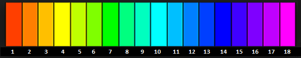
The color coding applied uses a predefined color scheme, named “simple”. Alternatively, you can use “Rainbow”:
p.colorScheme("Rainbow")
map.clear()
map.zoomToImageExtent(p)
tlayer = map.addLayer(p.toLayer())
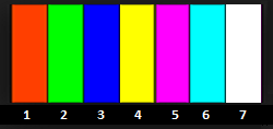
The simple palette is defined as follows with x denoting the value of the divider:
| Decimal | Binary | Color code |
|---|---|---|
| 1x | 001 | Red |
| 2x | 010 | Green |
| 3x | 011 | Red+Green=**Yellow** |
| 4x | 100 | Blue |
| 5x | 101 | Red+Blue=**Magenta** |
| 6x | 110 | Green+Blue=**Cyan** |
| 7x | 111 | Red+Green+Blue=**White** |
For example, if the divider is 2, all pixels displayed in white (which is the 7th color of the palette) are zones where 14 (that is 7 multiplied by 2) or more images are available.
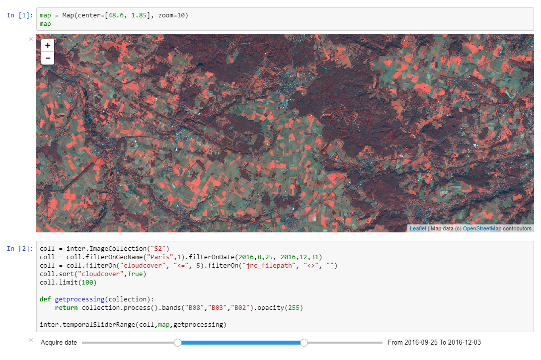
Temporal sliders
Temporal sliders can help in displaying all available acquisition dates for a specific Sentinel 2 images collection. To display the slider (created by using ipyWidgets) a call to the inter.temporalSlider method is used, that requires as arguments:
- the collection object;
- the map where the images have to be displayed;
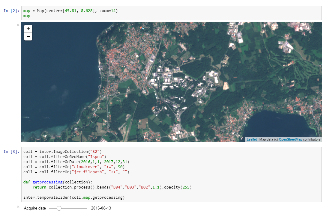
- the name of a python function to be used as callback. This function will receive as argument a reference to the collection element and has to return a processing element to be displayed on the map. In this example a True Color RGB composition is returned by the getprocessing python function.
map = Map(center=[45.81, 8.628], zoom=14)
map
coll = inter.ImageCollection("S2")
coll = coll.filterOnGeoName("Ispra")
coll = coll.filterOnDate(2016,1,1, 2017,12,31)
coll = coll.filterOn("cloudcoverpercentage", "<=", 5)
coll = coll.filterOn("jrc_filepath", "<>", "")

def getprocessing(collection):
    return collection.process().bands("B04","B03","B02",1.1).opacity(255)

inter.temporalSlider(coll,map,getprocessing)
By operating on the slider a single acquisition day is selected and the corresponding images are displayed on the map.
Temporal sliders can also help in displaying all available acquisition dates for a specific Sentinel 2 images collection. In this case the slider allows for the selection of a range of acquisition dates: