ImageProcess class¶

class inter.ImageProcess¶

ImageProcess class defines a processing chain object. It can be created from a filtered ImageCollection instance by calling the method ImageCollection.process(). Processing steps that perform specific transformation of the source data can be added to the processing chain. To visualize the ImageProcess object it can be added as a layer to a Map instance.

Examples:

A simple processing chain that selects the first band of the Core003 ImageCollection:

coll = inter.ImageCollection("C03")
p = coll.process()
p = p.band("1")

A more complex processing chain generated from a Sentinel2 ImageCollection:

Creation of an ImageCollection of images that cover Munchen(DE) and have small cloud cover:
coll = inter.ImageCollection("S2")
coll = coll.filterOnGeoName("Munchen", 0, "DE")
coll = coll.filterOnDate(2015,1,1, 2016,12,31)
coll = coll.filterOn("cloudcover", "<=", 5)
coll = coll.filterOn("jrc_filepath", "<>", "")
coll.limit(4)
coll.sort("cloudcover",True)
Generation of the ImageProcess object, selection of an RGB true-color composition (bands B04,B03,B02) and addition of the processing chain as a layer to the map:
p = coll.process().bands("B04","B03","B02",2)
map.zoomToImageExtent(p)
map.addLayer(p.toLayer())       

An example involving band maths (making the average of bands B04 and B03 masking out small values and applying a custom color scheme):

p1 = coll.process().band("B04")
p2 = coll.process().band("B03")
p1 = p1.math("+",p2).math("*",0.5).maskLT(600)
p1.scale(600,1500)
colors = ["Green", "Yellow", "Red"]
p1.colorCustom(colors)
p1.opacity(255)
map.clear()
map.addLayer(p1.toLayer())

Notes:

The calls to ImageProcess methods can be chained together using the . syntax. When more than one method is called in a single instruction, it is always a good practice to assign the result of the calls to a variable (or to the same process object) like in:

p1 = p1.math("+",p2).math("*",0.5).maskLT(600)

If a single method is called, it is perfecly safe to call without the assignment, like in:

p1.opacity(255)

General methods¶

ImageProcess.copyTo(imgProc)¶

Copies the content of an ImageProcess instance to another instance.

Args:

imgProc (ImageProcess): Destination instance of ImageProcess copyTo operation.

Example:

The following code shows a typical usage of copyTo method to obtain a copy of an existing ImageProcess istance and modify it:

# ImageCollection on Core003 dataset
coll = inter.ImageCollection("C03")

# Create a process object on band 1 , copy it and modify to work on all 3 bands
p1 = coll.process().band("1")
p2 = inter.ImageProcess()
p1.copyTo(p2)

# Modify the second processing chain to work on 3 bands
p2.bands()

# print number of bands in the original and the copied ImageProcess
print p1.numBands()
print p2.numBands()

ImageProcess.parameter(Name, Value)¶

Sets the value for a parameter of the ImageProcess object. Every type of ImageProcess object support a specific list of parameters, depending on the characteristics of the ImageCollection from which they are created.

Args:

Name (string): Name of the parameter.
Value (string): value to assign to the parameter.

Returns:

A reference to the modified instance of ImageProcess (so that this method can be chained with other methods using the . syntax).

Notes:

Here is the list of parameters implemented by the different types of ImageProcess objects:

ImageProcess created from ImageCollection of type “S2”:

interpolate values can be nearest, bilinear, cubic, cubicspline, lanczos, average, mode (default=nearest)

CloudMask values can be true, false (default=false). If true the GML cloud mask is displayed.

CloudProb values can be true, false (default=false). If true the cloud probability for L2A products or GML cloud mask for L1C products is displayed.

SceneClass values can be true, false (default=false). If true the Scene Classification for L2A products is displayed (see s2scl() function for the visualization legend)

ImageProcess created from ImageCollection of type “C03”:

mode values can be seamline or feathering (default=feathering)

interpolate values can be nearest, bilinear, cubic, cubicspline, lanczos, average, mode (default=nearest)

ImageProcess created from ImageCollection of type “DEM”:

source values can be SRTM, GEBCO or EUDEM (default=EUDEM).

mode values can be hillshade or dem (default=dem). If hillshade is selected, all following parameters can be used to customize how the hillshading is calculated.

azimuth solar azimuth angle i.e. the azimuth angle of the sun. It defines in which direction the sun is. Values can be from 0=West to 90=North, 180=East, etc. (default=45, NorthWest).

elevation solar elevation angle i.e. the altitude of the Sun over the horizon . Values can be from 0=horizon to 90=zenith (default=45).

lighting illumination coefficient. Values can be from 0.0 to 100.0 (default=1.2).

wslope weight to assign to the slope component. Values can be from 0.0 to 100.0 (default=1.0).

wshade weight to assign to the shading component. Values can be from 0.0 to 100.0 (default=1.0).

wcolor weight to assign to the color component. Values can be from 0.0 to 100.0 (default=1.0).

zfactor value to premultiply all elevation data. Values can be from 0.0 to 100.0 (default=1.0).

interpolate values can be nearest, bilinear, cubic, cubicspline, lanczos, average, mode (default=nearest)

ImageProcess created from ImageCollection of type “GHSL”:

none

ImageProcess created from ImageCollection of type “NDVI”:

none

ImageProcess created from ImageCollection of type “S1Mosaic”:

none

ImageProcess created from ImageCollection of type “GSW”:

mode values can be change, extent, recurrence, seasonality, transitions or occurrence (default=occurrence).

ImageProcess created from ImageCollection of type “CORINE”:

none
ImageProcess created from ImageCollection of type “BASEMAP”:
basemap values can be any integer value (written as a string) between “1” and “27” (default=”1”, Open Street Map). To have a list of all the available basemaps the method Map.printAvailableBasemaps() can be called.
modisdate (date as string in ‘YYYY-MM-DD’ format): For all MODIS basemaps (basemap from “21” to “25”) it is possible to select a specific date (default is yesterday).
Example:
p = inter.ImageCollection("BASEMAP").process()
p.parameter("basemap","21")
p.parameter("modisdate","2017-09-21")
ImageProcess created from a call to VectorLayer.process() method:

identify values can be all or first. It controls if the identify operation will return all features or only the first one (default=first).

identifyField values can be the empty string or a list of names of attributes of the vector layer (separated by blank character). In the first case, the identify operation returns all the attribute names and values of the selected features. If one or more names of attributes are given, then the identify operation will return only the values of those attributes separated with the “identifySeparator” if more than one feature is selected (default=empty string).

identifySeparator separator to put between values when the identify returns value on a single field, i.e. when identifyField is not empty (default=”#”).

identifyFilter filter on attributes to limit the features to identify. It can be a clause like AttributeName = value (default=empty string).

identifySortField name of the attribute to use to sort the identify results. It can be the empty string or the name of an attribute. In this second case, the results of an identify will be sorted in ascending mode on the values of the selected attribute (default=empty string).

All types of ImageProcess objects:

colorinterpolate values can be YES, NO (default=true)

ImageProcess.toLayer()¶

Saves the ImageProcess object to the server side processing chain DB and returns a string containing the unique ID of the processing chain itself. Passing the returned value to the Map.addLayer() method will add a layer to the map to display the processing chain.

Example:

Create a map instance:
map = Map()
map
Create a simple processing chain from Core003 dataset and add it as a new layer to the map:
p = inter.ImageCollection("C03").process()
map.addLayer(p.toLayer())

Returns:: A string containing the unique ID of the processing chain.

Bands selection¶

Methods in this group define what are the bands on which the ImageProcess object will operate. Bands can be the original bands of the source images or more complex (‘derived’) bands calculated from original bands.

ImageProcess.band(*args)¶

Sets the processing chain to work on a single band. To obtain the list of all available bands for an instance of ImageCollection the method ImageCollection.printBandNames() can be called. If an empty string or a non-existing band name is passed as an argument to the band method, usually the first available band from the source ImageCollection is used.

Args:

In case the processing chain is a standard processing chain, the band method has to be called by passing the name of the band (as obtained by calling the method ImageCollection.printBandNames())

BandName (string): Name of the band to work on (optional)

ScalingFactor (float): How many “standard deviation” around the mean value of the band should be considered for scaling band original values to BYTE for visualization. The values in the range [mean - ScalingFactor*StdDev, mean + ScalingFactor*StdDev] are linearly mapped to the range [0,255] (optional, default = 2.0)

In case the processing chain is a multi-band processing chain (see ImageProcess.multi()), the band method has to be called by passing the index of the band.

BandIndex (integer): Index of the band to display in the [1,n] range, beeing n the number of bands of the multi-band composition.

Returns:

A reference to the modified instance of ImageProcess (so that this method can be chained with other methods using the . syntax).

Example:

A simple example of usage of the band method for a standard processing chain and for a multi-band processing chain:

Create the map instance:
map = Map()
map
Create three instances of ImageProcess, one for each of the three bands of the Core003 ImageCollection:
p1 = inter.ImageCollection("C03").process().band("1")
p2 = inter.ImageCollection("C03").process().band("2")
p3 = inter.ImageCollection("C03").process().band("3")
Create an empty ImageProcess and call multi method with the correct ordering and then call band method to display only the second band:
p = inter.ImageProcess()
bands = [p1, p2, p3]
p = p.multi(bands).band(2)
map.addLayer(p.toLayer())

ImageProcess.bands(*args)¶

Sets the processing chain to work on an RGB composition of three bands. To obtain the list of all available bands for an instance of ImageCollection the method ImageCollection.printBandNames() can be called. If empty strings or a non-existing band name is passed as an argument to the bands method, usually the first available bands from the source ImageCollection are used.

Args:

In case the processing chain is a standard processing chain, the bands method has to be called by passing the names of the bands (as obtained by calling the method ImageCollection.printBandNames())

RBandName (string): Name of the band for the red channel (optional)

GBandName (string): Name of the band for the green channel (optional)

BBandName (string): Name of the band for the blue channel (optional)

ScalingFactor (float): How many “standard deviation” around the mean value of the band should be considered for scaling band original values to BYTE for visualization. The values in the range [mean - ScalingFactor*StdDev, mean + ScalingFactor*StdDev] are linearly mapped to the range [0,255] (optional, default = 2.0)

As an alternative, instead of the names of the three bands, it is possible to pass the name of a standard band combination, for instance one of the values inter.S2_* for Sentinel-2 products (use <tab> key to automatically expand the available names)

Predefined Sentinel-2 band combinations names and their correspondant bands:

Name	Red band	Green band	Blue band
S2_NaturalColors	B04	B03	B02
S2_FalseColorInfrared	B08	B04	B03
S2_FalseColorUrban	B12	B11	B04
S2_Agriculture	B11	B08	B02
S2_AtmosphericPenetration	B12	B11	B8A
S2_HealthyVegetation	B08	B11	B02
S2_LandWater	B08	B11	B04
S2_NaturalColorsWithAtmosphericRemoval	B12	B08	B03
S2_ShortwaveInfrared	B12	B08	B04
S2_VegetationAnalysis	B11	B08	B04
S2_Geology	B12	B04	B02
S2_Bathymetric	B04	B03	B01
S2_SWIR	B12	B8A	B04

In case the processing chain is a multi-band processing chain (see ImageProcess.multi()), the bands method has to be called by passing the indexes of the bands in the [0,n-1] range, beeing n the number of bands of the multi-band composition.

indexR (integer): index of the band to display in the Red channel.

indexG (integer): index of the band to display in the Green channel.

indexB (integer): index of the band to display in the Blue channel.

ScalingFactor (float): How many “standard deviation” around the mean value of the band should be considered for scaling band original values to BYTE for visualization. The values in the range [mean - ScalingFactor*StdDev, mean + ScalingFactor*StdDev] are linearly mapped to the range [0,255] (optional, default = 2.0)

Returns:

A reference to the modified instance of ImageProcess (so that this method can be chained with other methods using the . syntax).

Example:

A simple example of usage of the bands method for a multi-band processing chain: use the Core003 dataset and exchange two of the bands to obtain a false-color visualization:

Create the map instance:
map = Map()
map
Create three instances of ImageProcess, one for each of the three bands of the Core003 ImageCollection:
p1 = inter.ImageCollection("C03").process().band("1")
p2 = inter.ImageCollection("C03").process().band("2")
p3 = inter.ImageCollection("C03").process().band("3")
Create an empty ImageProcess and call multi method with the correct ordering and then call bands with a different ordering of the bands, then display the result on the map:
p = inter.ImageProcess()
bands = [p1, p2, p3]
p = p.multi(bands).bands(1,0,2)
map.addLayer(p.toLayer())

An example of using standard band combinations for Sentinel-2 display:

Create the map instance:

map = Map()
map

Create an ImageCollection and an ImageProcess:

coll = inter.ImageCollection("S2")
coll = coll.filterOnGeoName("Ispra")
coll = coll.filterOnDay(2017,10,14)
coll = coll.filterOn("cloudcover", "<=", 50)
coll = coll.filterOn("jrc_filepath", "<>", "")
p = coll.process()

Select a standard band combination and add the layer to the map:

p.bands(inter.S2_HealthyVegetation)

map.clear()
map.addLayer(p.toLayer())

ImageProcess.quicklooks()¶

Sets the processing chain to display the quicklooks of the collection, if available.

Returns:: A reference to the modified instance of ImageProcess (so that this method can be chained with other methods using the . syntax).

ImageProcess.count(BandName='', Divider=1.0)¶

Sets the processing chain to work on a derived band that calculates, for each pixel, the total number of overlapping valid pixels inside the ImageCollection instance from which the ImageProcess object is created. It is useful in order to have a visual representation of the consistency of an ImageCollection, especially for datasets like Sentinel2 where many images are available for the same geographic location.

Args:

BandName (string): Name of the band to work on (optional)
Divider (float): The real pixel-by-pixel count will be divided by this amount (optional, default = 1.0)

Returns:

A reference to the modified instance of ImageProcess (so that this method can be chained with other methods using the . syntax).

Example:

Arguments of the count() method are the name of a band and a divider. Then a color coding is applied using a predefined color scheme named “simple”. The simple palette is defined as follows with x denoting the value of the divider: Red for x images, Green for 2x, Blue for 3x, Yellow for 4x, Magenta for 5x, Cyan for 6x, and White for 7x or more images. For example, if the divider is 2, all pixels displayed in white color (which is the 7th color of the palette) are zones where 14 (that is 7 multiplyed by 2) or more images are available.

Create a map instance:

map = Map()
map

Create a Sentinel 2 ImageCollection and select the Sardegna region:

coll = inter.ImageCollection("S2")
coll = coll.filterOnGeoName("Sardegna")
coll = coll.filterOnDate(2016,7,1, 2016,9,30)
coll = coll.filterOn("cloudcover", "<=", 5)
coll = coll.filterOn("jrc_filepath", "<>", "")

Create a processing chain from the collection and select the count method on the B11 band with divider 1:

p = coll.process().count("B11",1)

Apply a color scheme and display the processing chain on the map:

p.colorScheme("Simple")
map.zoomToImageExtent(p)
map.addLayer(p.toLayer())

ImageProcess.normalizedDifference(BandName1='', BandName2='')¶

Sets the processing chain to work on a derived band that calculates, for each pixel, the normalized difference index between two bands of the source images. This is the basic function to calculate indexes like NDVI (that can be also calculated using ImageProcess:NDVI() and related methods). Written mathematically, the formula is: normalizedDifference = (BandName1-BandName2)/(BandName1+BandName2). To calculate the standard NDVI index, the BandName1 should be the name of the near infrared band (i.e. B08 for Sentinel 2 products), while BandName2 should be the name of the red visible band (i.e. B04 for Sentinel 2 products).

Args:

BandName1 (string): Name of the first band to use for calculation of the normalized difference index (optional).
BandName2 (string): Name of the second band to use for calculation of the normalized difference index (optional).

Example:

Create a map instance and center the visualization on the Netherlands:

map = Map(center=[52.2, 5.2], size=[800, 600], zoom=7)
map

Create a Sentinel 2 ImageCollection and select the Amsterdam region:

coll = inter.ImageCollection("S2")
coll = coll.filterOnGeoName("Amsterdam, Netherlands", 0.5)
coll = coll.filterOnDate(2016,12,1, 2016,12,30)
coll = coll.filterOn("cloudcover", "<=", 10).filterOn("jrc_filepath", "<>", "").limit(20)
coll.sort("cloudcover",True)

Create a processing chain from the collection, calculate the normalized difference between B08 and B04 bands (calculated values are in the range [0,65535]), then mask out all values less that 46000 then scale all values in the range [46000,55000] to the display range [0,255]:

p = coll.process().normalizedDifference("B08","B04").maskLT(46000.0).scale(46000,55000)

Apply a custom color scheme (created from a python list of colors) and display the processing chain on the map (the highest values of the index will be displayed in green color):

colors = ["Red", "Yellow", "Green"]
p.colorCustom(colors)
map.zoomToImageExtent(p)
map.addLayer(p.toLayer())

Returns:

A reference to the modified instance of ImageProcess (so that this method can be chained with other methods using the . syntax).

ImageProcess.NDVI()¶

Sets the processing chain to work on a derived band that calculates, for each pixel, the NDVI index (Normalized Difference Vegetation Index) between near-infrared band and red band of the source images: (NIR-RED)/(NIR+RED). The calculated values are in the range [0,65535]. This method is implemented only for ImageCollections that contain multi band images (i.e. Sentinel 2).

Returns:: A reference to the modified instance of ImageProcess (so that this method can be chained with other methods using the . syntax).

ImageProcess.GNDVI()¶

Sets the processing chain to work on a derived band that calculates, for each pixel, the GNDVI index (Green Normalized Difference Vegetation Index) defined as (NIR-GREEN)/(NIR+GREEN). The calculated values are in the range [0,65535]. This method is implemented only for ImageCollections that contain multi band images (i.e. Sentinel 2).

Returns:: A reference to the modified instance of ImageProcess (so that this method can be chained with other methods using the . syntax).

ImageProcess.BNDVI()¶

Sets the processing chain to work on a derived band that calculates, for each pixel, the BNDVI index (Blue Normalized Difference Vegetation Index) defined as (NIR-BLUE)/(NIR+BLUE). The calculated values are in the range [0,65535]. This method is implemented only for ImageCollections that contain multi band images (i.e. Sentinel 2).

Returns:: A reference to the modified instance of ImageProcess (so that this method can be chained with other methods using the . syntax).

ImageProcess.NBR()¶

Sets the processing chain to work on a derived band that calculates, for each pixel, the NBR index (Normalized Burn Ratio Index) defined as (NIR-SWIR2)/(NIR+SWIR2). The calculated values are in the range [0,65535]. This method is implemented only for ImageCollections that contain multi band images (i.e. Sentinel 2).

Returns:: A reference to the modified instance of ImageProcess (so that this method can be chained with other methods using the . syntax).

ImageProcess.NDSII()¶

Sets the processing chain to work on a derived band that calculates, for each pixel, the NDSII index (Normalized Difference Snow/Ice Index) defined as (GREEN-SWIR1)/(GREEN+SWIR1). The calculated values are in the range [0,65535]. This method is implemented only for ImageCollections that contain multi band images (i.e. Sentinel 2).

Returns:: A reference to the modified instance of ImageProcess (so that this method can be chained with other methods using the . syntax).

ImageProcess.NDWI()¶

Sets the processing chain to work on a derived band that calculates, for each pixel, the NDWI index (Normalized Difference Water Index) defined as (NIR-SWIR1)/(NIR+SWIR1). The calculated values are in the range [0,65535]. This method is implemented only for ImageCollections that contain multi band images (i.e. Sentinel 2).

Returns:: A reference to the modified instance of ImageProcess (so that this method can be chained with other methods using the . syntax).

ImageProcess.NDSI()¶

Sets the processing chain to work on a derived band that calculates, for each pixel, the NDSI index (Normalized Difference Salinity Index) defined as (SWIR1-SWIR2)/(SWIR1+SWIR2). The calculated values are in the range [0,65535]. This method is implemented only for ImageCollections that contain multi band images (i.e. Sentinel 2).

Returns:: A reference to the modified instance of ImageProcess (so that this method can be chained with other methods using the . syntax).

ImageProcess.NDSI2()¶

Sets the processing chain to work on a derived band that calculates, for each pixel, the NDSI2 index (Normalized Difference Salinity Index 2) defined as (RED-NIR)/(RED+NIR). The calculated values are in the range [0,65535]. This method is implemented only for ImageCollections that contain multi band images (i.e. Sentinel 2).

Returns:: A reference to the modified instance of ImageProcess (so that this method can be chained with other methods using the . syntax).

Controlling display¶

ImageProcess.scale(*args)¶

Sets the scaling values to convert data from their original range to [0,255] before being visualized on the map.

Args:

Scaling values that define the range can be specified using different methods:

Scaling based on the mean value of the input bands:
- factor (float): How many “standard deviation” around the mean value of the band should be considered for scaling band original values to BYTE for visualization. The values in the range [mean - ScalingFactor*StdDev, mean + ScalingFactor*StdDev] are linearly mapped to the range [0,255].
Scaling to a common range for all bands (the values in the range [Allmin,Allmax] for all bands are scaled to [0,255]):
- Allmin (float): minimum input value of the scaling range
- Allmax (float): maximum input value of the scaling range
Scaling to a different range for each band (the values in the range specific input range for a band are scaled to [0,255]):
- Rmin (float): minimum input value of the scaling range for the R band
- Rmax (float): maximum input value of the scaling range for the R band
- Gmin (float): minimum input value of the scaling range for the G band
- Gmax (float): maximum input value of the scaling range for the G band
- Bmin (float): minimum input value of the scaling range for the B band
- Bmax (float): maximum input value of the scaling range for the B band

Returns:

A reference to the modified instance of ImageProcess (so that this method can be chained with other methods using the . syntax).

Examples:

Scaling based on standard deviation and mean value of the selected images:
p.scale(2.0)
Scaling using the same range for all bands:
p.scale(100,2000)
Scaling using a different range for the three RGB bands:
p.scale(100,2000, 500,2000,  600,3000)

ImageProcess.noscale()¶

Disable the scaling operations so that the real image values are used to produce the visualization. Usually the scaling is disabled before a call to ImageProcess.colorMap() to set the colors to use for individual values of an image.

Returns:: A reference to the modified instance of ImageProcess (so that this method can be chained with other methods using the . syntax).

ImageProcess.shift(Value)¶

Quick way to change the scaling ranges previously set to increase or decrease luminosity of the visualization.

Args:

Value (float): Value to add to the input range definitions for the bands of the processing chain (those set with ImageProcess.scale() method). Use positive values to increase luminosity, negative values to decrease it.

Returns:

A reference to the modified instance of ImageProcess (so that this method can be chained with other methods using the . syntax).

ImageProcess.optimizeStats(Flag)¶

Sets the flag that controls if an homogeneization of input data values should be applied before visualization of ImageCollections that contain more than one source image. If enabled, image values are corrected based on difference from the average of averages of input bands.

Args:

Flag (boolean): True if the optimization has to be activated, False otherwise (default = False).

Returns:

A reference to the modified instance of ImageProcess (so that this method can be chained with other methods using the . syntax).

ImageProcess.opacity(Value)¶

Sets the opacity value to be used for the display of the processing chain as a layer into the Map instance.

Args:

Value (integer): Opacity to use for display from 0 = transparent to 255 = opaque (default = 255).

Returns:

A reference to the modified instance of ImageProcess (so that this method can be chained with other methods using the . syntax).

ImageProcess.colorScheme(*args)¶

Select one of the available color schemes to apply to a processing chain in order to convert values into colors used for display. To have the list of all available color schemes users can call the ImageCollection.printColorSchemes().

Args:

Name (string): Name of the color scheme to use for the display.
PutInFirstPosition (integer): Index of the color scheme colors to start with (optional, default = 0).

Returns:

A reference to the modified instance of ImageProcess (so that this method can be chained with other methods using the . syntax).

ImageProcess.colorCustom(List)¶

Defines a custom color scheme from a list of user defined colors. Colors can be defined both using their names (i.e. ‘green’) or using the web format (i.e. ‘#00FF00’)

Args:

List (python List of strings): List of strings containing names of color codes.

Example:

Typical usage of the colorCustom function is given in the following pieces of code.

Create the map instance:

map = Map()
map

Create an hillshading ImageProcess and set the colors from a list of colors:

p = inter.ImageCollection("DEM").process().parameter("mode","hillshade").scale(0,1500)
colors = ["#FFFFAA", "#27A827", "#0B8040", "Yellow", "#FFBA03", "#9E1E02", "#6E280A", "#8A5E42", "White"]
p.colorCustom(colors)
map.addLayer(p.toLayer())

Returns:

A reference to the modified instance of ImageProcess (so that this method can be chained with other methods using the . syntax).

ImageProcess.colorMap(*args)¶

Explicitly sets the colors for specific values of a single band image.

Args:

Colors (python dictionary): Dictionary containing image values as keys, and corresponding colors as values. Colors can be defined both using their names (i.e. ‘green’) or using the web format (i.e. ‘#00FF00’). All the values that are not present in the dictionary are considered no-data values.

Example:

Typical usage of the colorMap function is given in the following pieces of code.

Create a Map instance:

map = Map()
map

Select Sentinel-2 images covering Lombardia region:

coll = inter.ImageCollection("S2")
coll = coll.filterOnGeoName("Lombardia", 0, "IT")
coll = coll.filterOnDate(2018,1,1, 2018,4,30)
coll = coll.filterOn("cloudcover", "<=", 5)
coll = coll.filterOn("jrc_filepath", "<>", "")
coll = coll.filterOn("mgrs","like","32TNR")
coll.removeOverlap()
coll.sort("cloudcover",True)
coll.limit(10)

Classify the images on-the-fly using SVM algorithm:

modelsvm = 'model_svm.txt'

S2bands=["B02","B03","B04","B08"]
dictSVM={'model':modelsvm, 'method':'svm', 'band':[0,1,2,3]}
p = coll.processMulti(S2bands)
p = p.classify(dictSVM).band(0)

Disable scaling and set the colors to apply for each class:

p = p.noscale().colorMap({2: "red", 12: "yellow", 25: "green", 41: "blue", 50: "#000000" })

Information methods¶

ImageProcess.numBands()¶

Returns the number of bands selected for the instance of the processing chain using methods: band, bands, count, etc. In case of multi-band processing chain, the method returns the number of band of the overall chain, after all processing step have been applied.

Returns:: The number of bands of the ImageProcess instance.

ImageProcess.getCenterAndZoom()¶

Returns the extents of the geographic area covered by the processing chain expressed in (lat,lon) center point and zoom level.

Returns:: A python list containing three float values: [CenterLat CenterLon ZoomLevel].

ImageProcess.getDegreeExtents()¶

Returns the extents of the geographic area covered by the processing chain expressed in degrees (epsg = 4326).

Returns:: A python list containing four float values: [Lonmin Latmin Lonmax Latmax].

ImageProcess.getGoogleExtents()¶

Returns the extents of the geographic area covered by the processing chain expressed in coordinates in the Google Mercator reference system (epsg = 3857).

Returns:: A python list containing four float values: [xmin ymin xmax ymax].

ImageProcess.getWindowSize(minLongitude, minLatitude, maxLongitude, maxLatitude, zoomLevel)¶

Returns the dimension in pixels of the area covered by a rectangle (defined in (lat,lon) coordinates in EPSG 4326 and at a specific zoom level).

Args:

minLongitude (float): minimum longitude of the rectangle in degrees.
minLatitude (float): minimum latitude of the rectangle in degrees.
maxLongitude (float): maximum longitude of the rectangle in degrees.
maxLatitude (float): maximum latitude of the rectangle in degrees.
zoomLevel (integer): zoom level in the range [1,18].

Returns:

A python list containing two integer values: [width height].

ImageProcess.isTileBased()¶

Returns True if the processing chain can be queried in a tile-based mode from the server (display of the processing chain is done tile-by-tile using 256x256 tiles). Processing chains that contain only pixel-based processing steps can be queried in a tile-based mode. Processing chains that, for instance, contain the segmentation method labelAlphaCCs have to be queried in window-based mode (all the visible window is processed at the same time).

Returns:: True if the processing chain can be queried in a tile-based mode, False otherwise.

ImageProcess.printProcess()¶: Prints to the output of the notebook a detailed description of the processing chain, showing data members for all types of ImageProcess.

ImageProcess.identifyPoint(Longitude, Latitude, EPSG, ZoomLevel)¶

Given in input a point in a specific SRS, the method returns a string containing the values read from the processing chain related to that geographic location.

Args:

Longitude (float): Longitude of the query point.
Latitude (float): Latitude of the query point.
EPSG (integer): EPSG of the coordinate system in which the longitude and latitude coordinate are given.
ZoomLevel (integer): zoom level in the range [1,18] (used only for ImageProcess derived from VectorLayer instances to define the tolerance for searching vector features).

Returns:

A string containing information found at the specified geographic location inside the processing chain (value of pixels, elevation for DEM, etc.).

Processing steps¶

ImageProcess.maskLT(Value)¶

Processing step that performs a masking by substituting NoData to all values that are lower than the value passed as argument.

Args:

Value (float): Value to use as comparison: all values in the processing chain that are under this value are set to NoData.

Returns:

A reference to the modified instance of ImageProcess (so that this method can be chained with other methods using the . syntax).

ImageProcess.maskGT(Value)¶

Processing step that performs a masking by substituting NoData to all values that are greater than the value passed as argument.

Args:

Value (float): Value to use as comparison: all values in the processing chain that are over this value are set to NoData.

Returns:

A reference to the modified instance of ImageProcess (so that this method can be chained with other methods using the . syntax).

ImageProcess.maskBW(ValueMin, ValueMax)¶

Processing step that performs a masking by substituting NoData to all values that are inside the range defined by the two values passed as arguments.

Args:

ValueMin (float): Lower limit of the range.
ValueMax (float): Upper limit of the range.

Returns:

A reference to the modified instance of ImageProcess (so that this method can be chained with other methods using the . syntax).

ImageProcess.mask(imgProc)¶

Processing step that performs a masking by substituting NoData to all pixels that correspond to pixel 0 or Nodata in the ImageProcess instance passed as argument.

Args:

imgProc (ImageProcess): ImageProcess instance used as a comparison.

Returns:

A reference to the modified instance of ImageProcess (so that this method can be chained with other methods using the . syntax).

ImageProcess.invmask(imgProc)¶

Processing step that performs an inverted masking by substituting NoData to all pixels that correspond to valid pixels in the ImageProcess instance passed as argument.

Args:

imgProc (ImageProcess): ImageProcess instance used as a comparison.

Returns:

A reference to the modified instance of ImageProcess (so that this method can be chained with other methods using the . syntax).

ImageProcess.math(*args)¶

Processing step that performs a simple mathematical operation (sum, substract, multiply, divide, etc.) using as operand a scalar or another ImageProcess instance.

Args:

To perform a mathematical operation with a scalar:

Operator (string): Mathematical operator to apply. Possible values are: “+”, “-“, “*”, “/”.

Value (float): Scalar value to use in the mathematical operation.

To perform a mathematical operation with another ImageProcess instance:

Operator (string): Mathematical operator to apply. Possible values are: “+”, “-“, “*”, “/”.

imgProc (float): ImageProcess instance to be used as operand in the mathematical operation.

Returns:

A reference to the modified instance of ImageProcess (so that this method can be chained with other methods using the . syntax).

ImageProcess.blank(Value)¶

Processing step that sets all pixels to a specific value.

Args:

Value (float): Value to write on all the pixel of the ImageProcess instance.

Returns:

A reference to the modified instance of ImageProcess (so that this method can be chained with other methods using the . syntax).

ImageProcess.bitwise(Operator, imgProc)¶

Processing step that performs a bitwise operation using as operand a second instance of an ImageProcess.

Args:

Operator (string): Bitwise operator to apply. Possible values are: “AND”, “OR”, “XOR”, “NAND”.
imgProc (ImageProcess): ImageProcess instance used as operand.

Returns:

A reference to the modified instance of ImageProcess (so that this method can be chained with other methods using the . syntax).

ImageProcess.arith(*args)¶

Processing step that performs an arithmetic operation using as operand a scalar or another ImageProcess instance.

Args:

To perform an arithmetic operation with a scalar:

Operator (string): Arithmetic operator to apply. Possible operators are:

“ADD”

“SUB”

“MULT”

“DIV”

“INF”

“SUP”

“MASK”

“ADD_OVFL”

“SUB_OVFL”

“MULT_OVFL”

“CMP”

“ABSSUB”

“MASK2”

“SUBSWAP”

“SUBSWAP_OVFL”

“EQUAL”

“NDI”

Value (float): Scalar value to use in the mathematical operation.

To perform an arithmetic operation with another ImageProcess instance:

Operator (string): Arithmetic operator to apply. Possible values are the same that are listed in the previous section.

imgProc (float): ImageProcess instance to be used as operand in the mathematical operation.

Returns:

A reference to the modified instance of ImageProcess (so that this method can be chained with other methods using the . syntax).

ImageProcess.modulo(Value)¶

Processing step that performs a modulo operation: every pixel is substituted by the remainder after division by the Value passed as argument.

Args:

Value (float): Value to use as divider in the modulo operation.

Returns:

A reference to the modified instance of ImageProcess (so that this method can be chained with other methods using the . syntax).

ImageProcess.erode()¶

Processing step that performs an erode operation using a 3x3 structuring element.

Returns:: A reference to the modified instance of ImageProcess (so that this method can be chained with other methods using the . syntax).

ImageProcess.dilate()¶

Processing step that performs a dilate operation using a 3x3 structuring element.

Returns:: A reference to the modified instance of ImageProcess (so that this method can be chained with other methods using the . syntax).

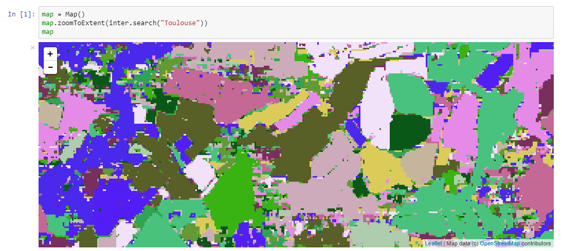
ImageProcess.labelAlphaCCs(Alpha, Omega)¶

Processing step that performs a constrained connectivity segmentation. The algorithm (described in Soille2008) relies on two constraints:

the local range threshold (called alpha);
the global range threshold (called omega).

The default parameter values are set to alpha = omega = 255. The constrained connectivity segmentation produces the coarsest partition of the viewed map such that any two points of each segment of the partition (called connected component) can be linked by a path included in the connected component while the absolute difference of any two successive pixels along the path never exceeds the alpha. In addition, the difference between the largest and smallest value within the connected component does not exceed omega. By increasing/decreasing the values of alpha and/or omega coarser/finer partitions can be obtained. In the example below, the segmentation is obtained on band 4 of a S2 image with alpha set to 256 and omega to 512. These values are appropriate since the theoretical range of the reflectance values of a S2 image is set between 1 and 10,000. The segmentation returns a labelled image with each segment (i.e., connected component) set to a unique label value. Since the number of segments of the partition can be as large as the number of pixels of the viewed area, for display purposes, the modulo(256) function is called to force the label values to belong to the integer range [0,255]. Random colors are given to each resulting 256 values by applying the color scheme “random”.

Args:

Alpha (float): Value to use as local range threshold.
Omega (float): Value to use as global range threshold.

Returns:

A reference to the modified instance of ImageProcess (so that this method can be chained with other methods using the . syntax).

Notes:

The labelAlphaCCs processing step is the first example of a non pixel-based operator. Whenever a processing chains has labelAlphaCCs step inside, the entire chain becomes WindowBased and the display is done not in TileBased mode but on the entire visible window at every pan and zoom done by the user on the Map.

Example:

Create the map instance and zoom to the city of Toulouse (see search() global function):
map = Map()
map.zoomToExtent(inter.search("Toulouse"))
map
Create an ImageCollection from 2017 Sentinel2 cloud free images:
coll = inter.ImageCollection("S2")
coll = coll.filterOnGeoName("Toulouse")
coll = coll.filterOnDate(2017,7,1, 2017,12,31)
coll = coll.filterOn("cloudcover", "<=", 0)
coll = coll.filterOn("jrc_filepath", "<>", "")
coll.limit(100)
coll.sort("cloudcover",True)
Create a processing chain that calculates the segmentation and add as a layer to the map:
p = coll.process().band("B04").labelAlphaCCs(256,1024).modulo(256).opacity(255)
p.colorScheme("random")
map.clear()
map.addLayer(p.toLayer())
Example output produced by the example code:

ImageProcess.filter2d(*args)¶

Filter image in spatial domain performed on single or multi-band raster dataset.

Args: * dict (Python Dictionary) with key value pairs. Each key (a ‘quoted’ string) is separated from its value by a colon (:). The items are separated by commas and the dictionary is enclosed in curly braces. An empty dictionary without any items is written with just two curly braces, like this: {}. A value can be a list that is also separated by commas and enclosed in square brackets [].

Supported keys in the dict:

key	value
filter	filter function (see values for different filter types in tables below)
dx	filter kernel size in x, use odd values only (default is 3)
dy	filter kernel size in y, use odd values only (default is 3)
pad	Padding method for filtering (how to handle edge effects) Possible values are: symmetric (default), replicate, circular, zero (pad with 0)
otype	Data type for output image

Edge detection

filter	description
sobelx	Sobel operator in x direction
sobely	Sobel operator in y direction
sobelxy	Sobel operator in x and y direction
homog	binary value indicating if pixel is identical to all pixels in kernel
heterog	binary value indicating if pixel is different than all pixels in kernel

Morphological filters

Note

For a more comprehensive list morphological operators, please refer to advanced spatial morphological operators.

filter	description
dilate	morphological dilation
erode	morphological erosion
close	morpholigical closing (dilate+erode)
open	morpholigical opening (erode+dilate)

Note

You can use the optional key ‘class’ with a list value to take only these pixel values into account. For instance, use ‘class’:[255] to dilate clouds in the raster dataset that have been flagged with value 255. In addition, you can use a circular disc kernel (set the key ‘circular’ to True).

Statistical filters

filter	description
smoothnodata	smooth nodata values (set nodata option!)
nvalid	report number of valid (not nodata) values in window
median	perform a median filter
var	calculate variance in window
min	calculate minimum in window
max	calculate maximum in window
ismin	binary value indicating if pixel is minimum in kernel
ismax	binary value indicating if pixel is maximum in kernel
sum	calculate sum in window
mode	calculate the mode (only for categorical values)
mean	calculate mean in window
stdev	calculate standard deviation in window
percentile	calculate percentile value in window
proportion	calculate proportion in window

Note

You can specify the no data value for the smoothnodata filter with the extra key ‘nodata’ and a list of no data values. The interpolation type can be set with the key ‘interp’ (check complete list of values, removing the leading “gsl_interp”).

Wavelet filters

Perform a wavelet transform (or inverse) in spatial domain.

Note

The wavelet coefficients can be positive and negative. If the input raster dataset has an unsigned data type, make sure to set the output to a signed data type using the key ‘otype’.

You can use set the wavelet family with the key ‘family’ in the dictionary. The following wavelets are supported as values:

daubechies
daubechies_centered
haar
haar_centered
bspline
bspline_centered

filter	description
dwt	discrete wavelet transform
dwti	discrete inverse wavelet transform
dwt_cut	DWT approximation in spectral domain

Note

The filter ‘dwt_cut’ performs a forward and inverse transform, approximating the input signal. The approximation is performed by discarding a percentile of the wavelet coefficients that can be set with the key ‘threshold’. A threshold of 0 (default) retains all and a threshold of 50 discards the lower half of the wavelet coefficients.

Returns:: A reference to the modified instance of ImageProcess (so that this method can be chained with other methods using the . syntax).

ImageProcess.range(InputMin, InputMax, OutputMin=0.0, OuputMax=255.0)¶

Processing step that performs a linear stretching from an input range to an output range.

Args:

InputMin (float): Minimum value of the input range.
InputMax (float): Maximum value of the input range.
OutputMin (float): Minimum value of the output range (optional, default = 0.0).
OutputMax (float): Maximum value of the output range (optional, default = 255.0).

Returns:

A reference to the modified instance of ImageProcess (so that this method can be chained with other methods using the . syntax).

ImageProcess.max()¶

Processing step that calculates the maximum vale for a multi-band combination.

Note:: After max processing step is applied, the multi-band combination will have a single band.
Returns:: A reference to the modified instance of ImageProcess (so that this method can be chained with other methods using the . syntax).

ImageProcess.classify(*args)¶

Supervised classification of a raster dataset. The classifier must have been trained via the VectorOgr:train() method. The classifier can be selected with the key ‘method’ and possible values ‘svm’ and ‘ann’:

Args: * dict (Python Dictionary) with key value pairs. Each key (a ‘quoted’ string) is separated from its value by a colon (:). The items are separated by commas and the dictionary is enclosed in curly braces. An empty dictionary without any items is written with just two curly braces, like this: {}. A value can be a list that is also separated by commas and enclosed in square brackets [].

Returns:: A reference to the modified instance of ImageProcess (so that this method can be chained with other methods using the . syntax).

Supported keys in the dict (with more keys defined for the respective classication methods):

key	value
method	Classification method (svm or ann)
model	Model filename to save trained classifier
band	Band index (starting from 0). The band order must correspond to the band names defined in the model. Leave empty to use all bands

The support vector machine (SVM) supervised classifier is described here. The implementation in JIPlib is based on the open source libsvm.

The artificial neural network (ANN) supervised classifier is based on the back propagation model as introduced by D. E. Rumelhart, G. E. Hinton, and R. J. Williams (Nature, vol. 323, pp. 533-536, 1986). The implementation is based on the open source C++ library fann (http://leenissen.dk/fann/wp/).

Prior probabilities

Prior probabilities can be set for each of the classes. The prior probabilities can be provided with the key ‘prior’ and a list of values for each of the (in ascending order). The priors are automatically normalized by the algorithm. Alternatively, a prior probability can be provided for each pixel, using the key ‘priorimg’ and a value pointing to the path of multi-band raster dataset. The bands of the raster dataset represent the prior probabilities for each of the classes.

Classifying parts of the input raster dataset

Parts of the input raster dataset can be classified only by using a vector or raster mask. To apply a vector mask, use the key ‘extent’ with the path of the vector dataset as a value. Optionally, a spatial extent option can be provided with the key ‘eo’ that controlls the rasterization process (values can be either one of: ATTRIBUTE|CHUNKYSIZE|ALL_TOUCHED|BURN_VALUE_FROM|MERGE_ALG). For instance, you can define ‘eo’:’ATTRIBUTE=fieldname’ to rasterize only those features with an attribute equal to fieldname.

To apply a raster mask, use the key ‘mask’ with the path of the raster dataset as a value. Mask value(s) not to consider for classification can be set as a list value with the key ‘msknodata’.

key	value
extent	Data type for output image
eo	Special extent options controlling rasterization
mask	Only classify within specified mask
msknodata	Mask value(s) in mask not to consider for classification
nodata	Nodata value to put where image is masked as no data

ImageProcess.execute(*args, **kvargs)¶

Processing step that executes a custom python function inside the server-side loop of the processing chain. This method uses internally the python inspect module to obtain a string containing the python code, and passes it to the server-side parallel environment where a python interpreter is executed. The python function can access the input pixels and modify them in order to pass them to the subsequent step of the chain. In case of a single-band processing chain, the python function will find the input pixel values in a variable name img which will be a numpy bi-dimensional array. In order to change the pixels the function has to contain the instruction global img and apply some modification to the content of the img numpy array. In case of a multi-band processing chain (one that derives from the usage of ImageProcess.multi() method), the execute step can be performed in a band-by-band mode (each transformation on a band is independent from what is done on the other bands) or in a single-output mode (a single band is produced in output by processing all the input bands). In the first case (band-by-band mode) the python function works in the same way as the single-band processing chain (the input pixel values are in the img input numpy array and by using global img the function can modify the pixels). In the second case (single-ouput mode) the python function will find in variables named band0, band1, etc.. the input bands of the processing chain and it is expected to write the result in the img numpy array. The example session below will provide examples of both cases. The python function can have any number and type of input parameters. The call to execute method should be done by passing as first argument the python function, followed by all other parameters (ordered or by name). Inside the python function these libraries will be available for the creation of the output image: 1) numpy 2) scipy.ndimage 3) jiplib No import command is allowed inside the python function.

Args:

func (python function object): Python function to execute
*args, **kvargs: Input parameters to be passed in the call to the python function. These parameters can be passed both by oder and by key-value.
OptionalModificators: Parameters that influence the way the python function is executed. They can be any of this list of values:

Optional modificator	Effect on the processing chain execution
EXECUTE_Tile	Executes the python function on 256x256 tiles (DEFAULT)
EXECUTE_Window	Executes the python function on the visible window
EXECUTE_SingleOutput	A single band output is produced from all the input bands (DEFAULT)
EXECUTE_MultiOutput	The python function is called on a band-by-band mode
EXECUTE_Enlarge0	Process exactly the input area without any enlargement
EXECUTE_Enlarge1	Enlarge the processing area by 1 pixel for each side
EXECUTE_Enlarge2	Enlarge the processing area by 2 pixels for each side
EXECUTE_Enlarge3	Enlarge the processing area by 3 pixels for each side
EXECUTE_Enlarge4	Enlarge the processing area by 2 pixels for each side

Returns:

A reference to the modified instance of ImageProcess (so that this method can be chained with other methods using the . syntax).

Example

A simple masking performed with the server-side execute processing step.

Definition of a python function that works on a single band and uses numpy sintax to change any pixel of the input img array to 0 (correspending to the NO-DATA value) when the input pixel value is less or equal to the parameter n:
def maskless(n):
    global img
    img[img<=n] = 0
Definition of a python function that works on a single band and uses scipy.ndimage library to perform a gaussian blur:
def gauss(s=5):
    global img
    img = ndimage.gaussian_filter(img, sigma=s)
Creation of an ImageCollection:
coll = inter.ImageCollection("S2")
coll.filterOnPoint(8.6214,45.8198)
coll = coll.filterOnDay(2017,10,14)
coll = coll.filterOn("cloudcover", "<=", 50)
coll = coll.filterOn("jrc_filepath", "<>", "")
Creation of a processing chain starting from band B04 of the ImageCollection and concatenating two execute processing steps (since the gaussian blur is not a pixel-based operation, the EXECUTE_Window optional modificator is used):
p = coll.process().band("B04").execute(maskless,1000).execute(gauss,EXECUTE_Window,3)
Display of the result on the map:
map.clear()
map.addLayer(p.toLayer())
A more complex python function to create a simple algorithm to detect burnt area (stubble burning mapping)

Python function thet defines 5 optional arguments as thresholds on the input bands (with default values). The output img numpy array is initialized as an array containing all 1.0 values and having the same shape and data type of the input band0 (instruction numpy.ones_like). Then a masking on each of the four input bands sets to 0 (NO-DATA) all the pixels that are below or over the corresponding threshold:
def stubble(v4=1000, v6=1200, v8=1200, v11_1=500, v11_2=1600):
    global img
    img = numpy.ones_like(band0)
    img[band0>v4] = 0
    img[band1>v6] = 0
    img[band2>v8] = 0
    img[numpy.logical_or(band3<v11_1, band3>v11_2)] = 0
Creation of an ImageCollection:
coll = Collection(collections.EarthObservation.Copernicus.Sentinel2.Level1C)
coll = coll.filterOnDay(2016,7,13)
coll = coll.filterOnRect(23.5, 44.2, 23.8, 44.6)
Creation of an multi-band ImageProcess with four input bands:
bands = ["B04","B06","B08","B11"]
p = coll.processMulti(bands).execute(stubble).band(0).scale(0,1).colorCustom(["Lime"])
Display of the result on the map:
map.clear()
map.addLayer(p.toLayer())

Combine operations¶

Combine operators are a specific type of processing steps that are applied to R,G,B byte bands just before saving data to PNG format to send to the Map client.

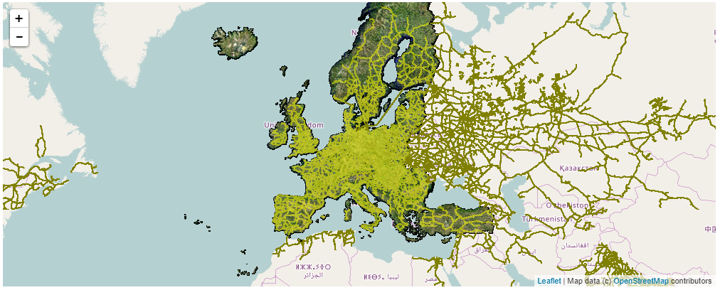
ImageProcess.blend(imgProc, OpacityValue)¶

Combine operation that blends together two R,G,B images using alpha values to generate a composite image. It can be used to create a unique ImageProcess from two distinct ones (for instance a base raster ImageProcess and an ImageProcess created from a VectorLayer instance)

Args:

imgProc (ImageProcess): Instance of the ImageProcess object to blend over.
OpacityValue (integer): Opacity of the overimposed ImageProcess (acceptable values in the range from 0 = transparent to 255 = opaque)

Returns:

A reference to the modified instance of ImageProcess (so that this method can be chained with other methods using the . syntax).

Example

Create the map instance:

map = Map()
map

Create an ImageProcess instance p from Core003 dataset:

p = inter.ImageCollection("C03").process()

Create an ImageProcess instance pv from a VectorLayer of the world railroads (colored in yellow):

v = inter.VectorLayer("railroads")
v.set('all','line','stroke','#ffff00')
pv = v.process()

Blend together p and pv and save the result in p (using half opacity):

p = p.blend(pv,128)
map.addLayer(p.toLayer())

Visualization produced by the example code:

Global operators¶

Global operators are processing steps that use other processing elements as input arguments to construct more complex processing chains.

ImageProcess.rgb(imgProcR, imgProcG, imgProcB)¶

Global operator that builds an RGB image by putting together three instances of ImageProcess class.

Args:

imgProcR (ImageProcess): Instance of the ImageProcess object to put in the Red band.
imgProcG (ImageProcess): Instance of the ImageProcess object to put in the Green band.
imgProcB (ImageProcess): Instance of the ImageProcess object to put in the Blue band.

Returns:

A reference to the modified instance of ImageProcess (so that this method can be chained with other methods using the . syntax).

Examples:

A simple example of usage of the rgb method: use the Core003 dataset and exchange two of the bands to obtain a false-color visualization:

Create the map instance:
map = Map()
map
Create three instances of ImageProcess, one for each of the three bands of the Core003 ImageCollection:
p1 = inter.ImageCollection("C03").process().band("1")
p2 = inter.ImageCollection("C03").process().band("2")
p3 = inter.ImageCollection("C03").process().band("3")
Create an empty ImageProcess and call rgb method with a different ordering of the bands, then display the result on the map:
p = inter.ImageProcess()
p.rgb(p2,p1,p3)
map.addLayer(p.toLayer())

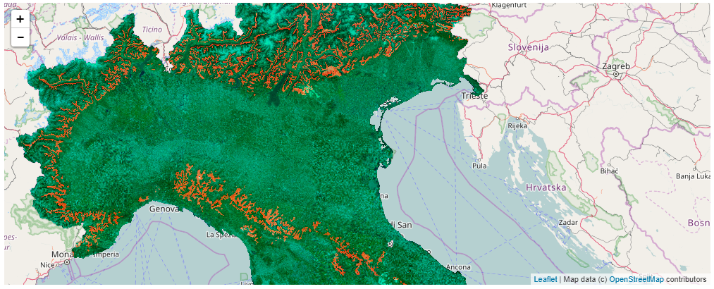
A more complex example: highlite a range of elevation (all areas between 900 and 1300 meters above sea level) inside Italy and display them in RGB mode with two bands of Core003 dataset:

Create the map instance:
map = Map()
map
Create two instances of ImageProcess, for the second and third band of the Core003 ImageCollection:
p2 = inter.ImageCollection("C03").process().band("2")
p3 = inter.ImageCollection("C03").process().band("3")
Create an instance of ImageProcess from DEM dataset by masking all values out of the elevation range [900,1300] meters above sea level:
pDEM = inter.ImageCollection("DEM").process().maskLT(900).maskGT(1300).range(0,1300,0,255)
Create an instance of ImageProcess from the nuts1 VectorLayer that visualizes only Italy:
v = inter.VectorLayer("nuts1").opacity(128)
v.remove('default','all')
country = "[ICC] = 'IT'"
v.set('default',country,'poly','fill','#ff000055')
pItaly = v.process()
Mask out all countries except Italy from the three ImageProcess instances:
p2.mask(pItaly)
p3.mask(pItaly)
pDEM.mask(pItaly)
Create an empty ImageProcess and call rgb method putting together the three bands, then display the result on the map:
p = inter.ImageProcess()
p.rgb(pDEM,p2,p3)
map.addLayer(p.toLayer())
Visualization produced by this last example code:

ImageProcess.multi(List)¶

Global operator that builds a multi-band image by putting together one or more instances of ImageProcess class.

Args:

List (python List of ImageProcess): List containing one or more instances of ImageProcess class.

Returns:

A reference to the modified instance of ImageProcess (so that this method can be chained with other methods using the . syntax).

Example:

A simple example of usage of the multi method: use the Core003 dataset and exchange two of the bands to obtain a false-color visualization:

Create the map instance:
map = Map()
map
Create three instances of ImageProcess, one for each of the three bands of the Core003 ImageCollection:
p1 = inter.ImageCollection("C03").process().band("1")
p2 = inter.ImageCollection("C03").process().band("2")
p3 = inter.ImageCollection("C03").process().band("3")
Create an empty ImageProcess and call multi method with a different ordering of the bands, then display the result on the map:
p = inter.ImageProcess()
bands = [p2, p1, p3]
p.multi(bands).bands(0,1,2)
map.addLayer(p.toLayer())

ImageProcess.addBand(imgProc)¶

Add a new band to an existing multi-band image.

Args:

imgProc (ImageProcess): ImageProcess instance to add.

Returns:

A reference to the modified instance of ImageProcess (so that this method can be chained with other methods using the . syntax).

Example:

A simple example of usage of the multi method: use the Core003 dataset and add a Corine band to it:

Create the map instance:
map = Map()
map
Create three instances of ImageProcess, one for each of the three bands of the Core003 ImageCollection:
p1 = inter.ImageCollection("C03").process().band("1")
p2 = inter.ImageCollection("C03").process().band("2")
p3 = inter.ImageCollection("C03").process().band("3")
p4 = inter.ImageCollection(collections.BaseData.Landcover.CLC2012).process().noscale().colorReset()
Create an empty ImageProcess and call multi with 3 bands, than add the Corine band and use it to display in RGB as the Blue band:
p = inter.ImageProcess()
bands = [p1, p2, p3]
p.multi(bands)
p.addBand(p4)
p.bands(0,1,3)
map.addLayer(p.toLayer())

Export functions¶

ImageProcess.exportPixelsX(minLongitude, minLatitude, maxLongitude, maxLatitude, zoomLevel)¶

Given a rectangle (defined in (lat,lon) coordinates in EPSG 4326 and at a specific zoom level), the method returns the number of pixel in the X axis for the export as an image or a numpy array.

Args:

minLongitude (float): minimum longitude of the rectangle in degrees.
minLatitude (float): minimum latitude of the rectangle in degrees.
maxLongitude (float): maximum longitude of the rectangle in degrees.
maxLatitude (float): maximum latitude of the rectangle in degrees.
zoomLevel (integer): zoom level in the range [1,18].

Returns:

Number of pixels in the X direction (width of the image or numpy array produced from the input rectangle).

ImageProcess.exportPixelsY(minLongitude, minLatitude, maxLongitude, maxLatitude, zoomLevel)¶

Given a rectangle (defined in (lat,lon) coordinates in EPSG 4326 and at a specific zoom level), the method returns the number of pixel in the Y axis for the export as an image or a numpy array.

Args:

minLongitude (float): minimum longitude of the rectangle in degrees.
minLatitude (float): minimum latitude of the rectangle in degrees.
maxLongitude (float): maximum longitude of the rectangle in degrees.
maxLatitude (float): maximum latitude of the rectangle in degrees.
zoomLevel (integer): zoom level in the range [1,18].

Returns:

Number of pixels in the Y direction (height of the image or numpy array produced from the input rectangle).

ImageProcess.exportNumBytes(minLongitude, minLatitude, maxLongitude, maxLatitude, zoomLevel)¶

Given a rectangle (defined in (lat,lon) coordinates in EPSG 4326 and at a specific zoom level), the method returns the number of bytes that the ImageProcess.exportImage() method will produce if called with the same input rectangle.

Args:

minLongitude (float): minimum longitude of the rectangle in degrees.
minLatitude (float): minimum latitude of the rectangle in degrees.
maxLongitude (float): maximum longitude of the rectangle in degrees.
maxLatitude (float): maximum latitude of the rectangle in degrees.
zoomLevel (integer): zoom level in the range [1,18].

Returns:

Number of bytes that the ImageProcess.exportImage() method will produce if called with the same input rectangle.

ImageProcess.exportCellsize(minLongitude, minLatitude, maxLongitude, maxLatitude, zoomLevel)¶

Given a rectangle (defined in (lat,lon) coordinates in EPSG 4326 and at a specific zoom level), the method returns the cellsize (spatial resolution) in Google Mercator projection of the TIFF file that the ImageProcess.exportImage() will produce if called with the same input rectangle.

Args:

minLongitude (float): minimum longitude of the rectangle in degrees.
minLatitude (float): minimum latitude of the rectangle in degrees.
maxLongitude (float): maximum longitude of the rectangle in degrees.
maxLatitude (float): maximum latitude of the rectangle in degrees.
zoomLevel (integer): zoom level in the range [1,18].

Returns:

Cellsize in Google Mercator projection of the TIFF file that the ImageProcess.exportImage() will produce if called with the same input rectangle.

ImageProcess.exportImage(minLongitude, minLatitude, maxLongitude, maxLatitude, zoomLevel, TiffFilePath)¶

Given a rectangle (defined in (lat,lon) coordinates in EPSG 4326 and at a specific zoom level), the method exports the processing chain to a georeferenced TIFF file. The path of the output file has to be a path relative to the special <home>/data folder where the output file will be created. Please note that the export could cause the creation of big files (use methods ImageProcess.exportPixelsX() and ImageProcess.exportPixelsY() to have width and height of the output image in pixels). In future version of the library the JEODPP infrastructure will set up a limit to the total number of pixels that can be exported and/or on the dimension of the file written to the local storage.

Args:

minLongitude (float): minimum longitude of the rectangle in degrees.
minLatitude (float): minimum latitude of the rectangle in degrees.
maxLongitude (float): maximum longitude of the rectangle in degrees.
maxLatitude (float): maximum latitude of the rectangle in degrees.
zoomLevel (integer): zoom level in the range [1,18].
TiffFilePath (string): path of the output file to produce in TIFF format (relative path from the <home>/data folder).

Returns:

True if the export is successful, False otherwise.

Example:

The following lines of code provide an example of exporting in TIFF format the Core003 over a part of Italy:

p = inter.ImageCollection("C03").process()

lonmin = 10
lonmax = 14

latmin = 40
latmax = 45

zoom = 8
outputfile = "italy8.tif"

print "cellsize = " , p.exportCellsize(lonmin,latmin,lonmax,latmax,zoom)
print "pixel in X = " , p.exportPixelsX(lonmin,latmin,lonmax,latmax,zoom)
print "pixel in Y = " , p.exportPixelsY(lonmin,latmin,lonmax,latmax,zoom)
print "number of bytes = " , p.exportNumBytes(lonmin,latmin,lonmax,latmax,zoom)

p.exportImage(lonmin,latmin,lonmax,latmax,zoom,outputfile)

ImageProcess.stats(minLongitude, minLatitude, maxLongitude, maxLatitude, zoomLevel, ScalingFactor)¶

Calculate and returns the statistics of the processing chain over the extent and zoom level passed as arguments.

Args:

minLongitude (float): minimum longitude of the rectangle in degrees.
minLatitude (float): minimum latitude of the rectangle in degrees.
maxLongitude (float): maximum longitude of the rectangle in degrees.
maxLatitude (float): maximum latitude of the rectangle in degrees.
zoomLevel (integer): zoom level in the range [1,18].
ScalingFactor (float): How many “standard deviation” around the mean value of the band should be considered for scaling band original values to BYTE for visualization. The values in the range [mean - ScalingFactor*StdDev, mean + ScalingFactor*StdDev] are linearly mapped to the range [0,255] (optional, default = 2.0)

Returns:

If the processing chain is a single-band processing chain, two values are returned: the min and max value to be used to scale the pixel values to convert to BYTE for visualization. If the processing chain is an RGB processing chain, two values are returned per each of the three bands (R, G, and B), six values in total: each couple of values contains the min and max value to be used to scale the pixel values to convert to BYTE for visualization. These values can be directly copy and pasted in the call to ImageProcess.scale() method.

Example:

Typical usage of the stats function is given in the following pieces of code:

Create the map instance and zoom to Ispra region:

map = Map(center=[45.81, 8.628], zoom=14)
map

Create a simple processing chain from Core003 dataset:

p = inter.ImageCollection("C03").process()

Get the statistics of the processing chain over a rectangular extent:

print p.stats(8,45,9,46,8, 2.0)

In order not to have a print with many decimal characters:

print [int(i) for i in p.stats(8,45,9,46,8, 2.0)]