Exploring other collections
In this notebook we will explore some other available collections. Items covered:
Very high spatial resolution European mosaic Core 03
The Core 03 mosaic has been created from 2.5 meters resolution SPOT images acquired in 2013-2014.
More information on Core_03 can be found on the Copernicus Space Component Data Access (CSCDA) website
This collection consists of two different mosaics:
- The first mosaic has been obtained by feathering adjacent images.
- The second mosaic is based on morphological image compositing, see also [Soi2014].
The mosaics can be selected with the process attribute “parameter”, setting the “mode” to “feathering” or “seamline” respectively:
coll = inter.ImageCollection("C03")
p = coll.process()
#p.parameter("mode","feathering")
p.parameter("mode","seamline")
map.clear()
tlayer = map.addLayer(p.toLayer())
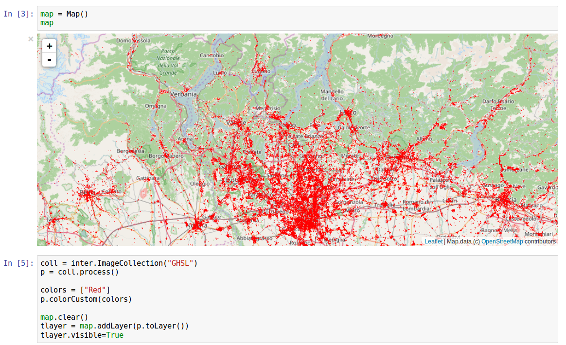
Global Human Settlement Layer
GHSL is a sample result dataset calculated by the Global Human Settlement project GHSL
The GHSL collection considered here is based on global processing of Sentinel-1 images performed on the JEODPP
As an example, we add the collection “GHSL” to a map, using a custom color (ImageProcess.colorCustom() with a single color (e.g, “Red”) that defines the human settlements:
coll = inter.ImageCollection("GHSL")
p = coll.process()

colors = ["Red"]
p.colorCustom(colors)

map.clear()
tlayer = map.addLayer(p.toLayer())
tlayer.visible=True
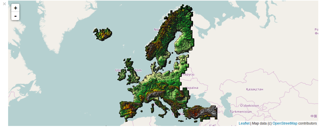
European Digital elevation model EU-DEM
The European Digital Elevation Model EU-DEM is a hybrid product based on SRTM and ASTER GDEM data fused by a weighted averaging approach. It is a realisation of the Copernicus programme, managed by the European Commission.
Its spatial resolution is at 25 m with vertical accuracy of +/- 7 meters RMSE.
The following parameters can be set to define how the display of DEMs is generated on-the-fly:
- “mode”: “hillshade” or “dem”;
- “azimuth”: sun azimuth in degrees (0 means west, 90 north, 180 east, etc…);
- “elevation”: sun elevation over the horizon in degrees;
- “lighting”: global illumination
- “wslope”: weight of the slope component that is added to the hillshading to increment the 3D effect;
- “wshade”: weight of the shade component;
- “wcolor”: weight of the color component;
- “zfactor”: the value to magnify the elevation.
We will use a Python tuple containing a list of colors to create a custom palette. The range of elevation values that correspond to the color range can be set using the p.scale() method. In this example all values below zero elevation are represented with the first color of the palette, while all values over elevation 1500 meters are represented with the last color of the palette.
Note that colors of the custom palette can be written in RGB mode (like “#27A827”) of with color names. The function coll.printNamedColors() gives the list of all available named colors with their corresponding RGB mode:
p = inter.ImageCollection("DEM").process()
p.parameter("source","EUDEM")
p.parameter("mode","hillshade")
p.scale(0,1500)
colors = ["#FFFFAA", "#27A827", "#0B8040", "Yellow", "#FFBA03", "#9E1E02", "#6E280A", "#8A5E42", "White"]
p.colorCustom(colors)
map.clear()
tlayer1 = map.addLayer(p.toLayer())
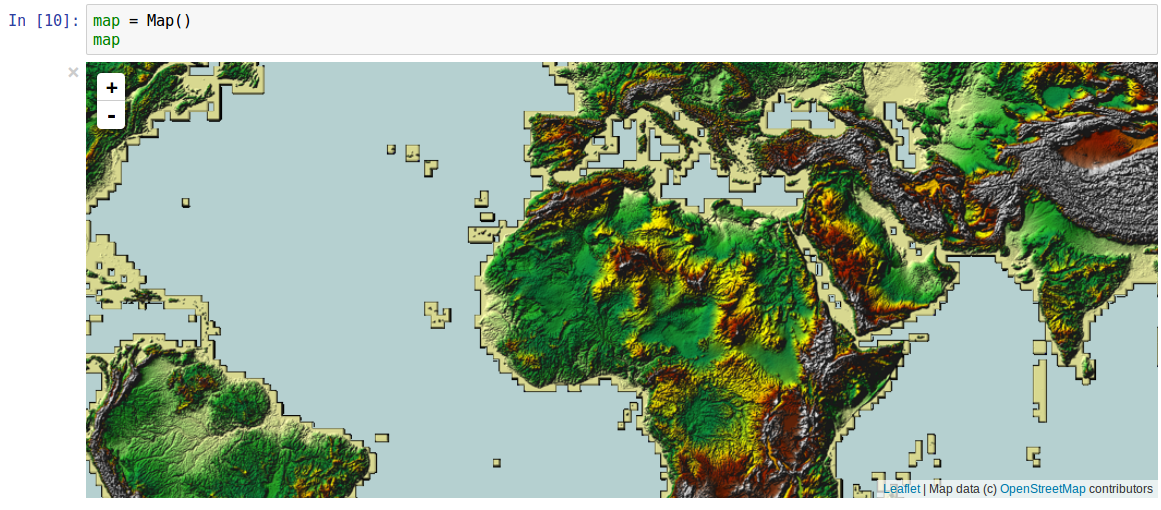
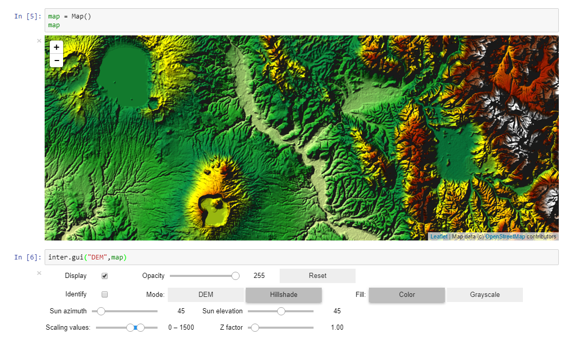
SRTM global Digital Elevation Model
Between 60° north and 56° south latitude, the SRTM 1 arc second DEM is available as a collection called SRTM.
Here we demonstrate the use of a graphical user interface (GUI) for setting the parameters that were introduced in the previous section on the EU-DEM. First create the map:
map = Map()
map
Then open the graphical interface to play with SRTM and the display settings:
inter.gui("SRTM",map)
See gui() for a description of the gui method.