Working with time series

In this tutorial we will explore time series, based on the NDVI time series obtained from SPOT-VEGETATION and PROBA-V.

NDVI time series collection

We create a map and a label, that will allow us to display pixel values for some location:

from ipywidgets import widgets
map = Map()
label = widgets.Label(layout=widgets.Layout(width='100%', max_width='1000px'))
widgets.VBox([map, label])

A time series of Normalised Difference Vegetation Index (NDVI) at 1km spatial resolution and 10 days temporal resolution is available from 1998 to 2013, based on satellite data acquired with the SPOT-VEGETATION (1 and 2) and PROBA-V sensors. This data is part of the Copernicus Global Land Service Products. The data are organised in a multi-band raster dataset and made available as a collection named “NDVI”.

The steps to display the NDVI time series as an RGB false color image are:

1. create a new collection object (coll), selecting the “NDVI” as the collection;
2. filter on date to select data from 2000-01-01 to 2001-07-28;
3. get familiar with the band names by using using coll.printBandNames();
4. create a new process object (p), creating an RGB false color image using the function bands(). Use the band names that represent the NDVI values for the dates 01/01/2000, 01/05/2000 and 01/09/2000;
5. add the layer of the process to the map above.

In code this is written as:

coll = inter.ImageCollection("NDVI")
coll = coll.filterOnDate(2000,1,1,2001,7,28)
p = coll.process().bands("2000_01_01","2000_05_01","2000_09_01")
map.clear()
tlayer = map.addLayer(p.toLayer())

In addition, we create an identifier object using the function identify(). The processing element is derived from the collection and displayed on the map, activating the identify marker to query the pixel values and output them to the label:

mark = inter.identify(map,p,label)

Animating time series with temporal slider

We will create a special temporal slider with an animate function

coll = inter.ImageCollection("NDVI")
coll = coll.filterOnDate(2000,1,1,2001,7,28)
def getprocessing(collection):
    p = collection.process()
    collection.printBandNames()
    return p

inter.temporalSliderAnimate(coll,map,getprocessing,2000)

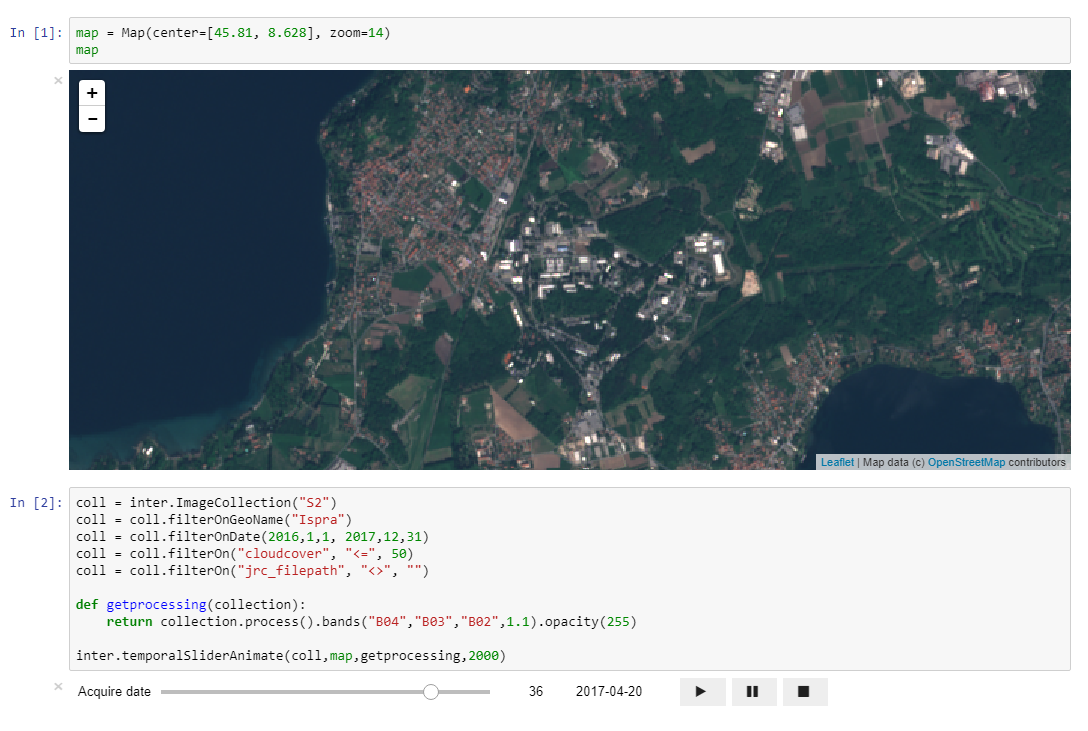
The function temporalSliderAnimate() expects four arguments:

1. collection: the NDVI time series collection we introduced above;
2. map: the map on which we display the animation;
3. call back function to set the start acquisition date of the slider (getprocessing);
4. Interval in milliseconds to wait before passing to the following date.

We can add a custom color palette to the process in the call back function. For instance, use the color palette: colors = [“Red”, “Orange”, “Yellow”, “Green”, “#005500”]:

coll = inter.ImageCollection("NDVI")
coll = coll.filterOnDate(2000,1,1,2001,7,28)
def getprocessing(collection):
    p = collection.process()
    collection.printBandNames()
    colors = ["Red", "Orange", "Yellow", "Green", "#005500"]
    p.colorCustom(colors)
    return p
inter.temporalSliderAnimate(coll,map,getprocessing,2000)

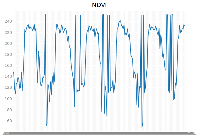
Plot NDVI time series data as a function

When visualising time series in a map, you are restricted to single date snapshots, RGB false colors of three selected dates. In the example above, we introduced the animation. However, it is often interesting to have an overview of the full time series for single pixel as a function.

We will introduce a marker in our map that can be dragged and dopped on a location, for which the entire time series are extracted. The extracted array of pixel values is then plot on a graph, using the bqplot module.

We will first filter the collection with NDVI time series on date, selecting the values between January 2000 and July 2005:

coll = inter.ImageCollection("NDVI")
coll = coll.filterOnDate(2000,1,1,2005,7,31)

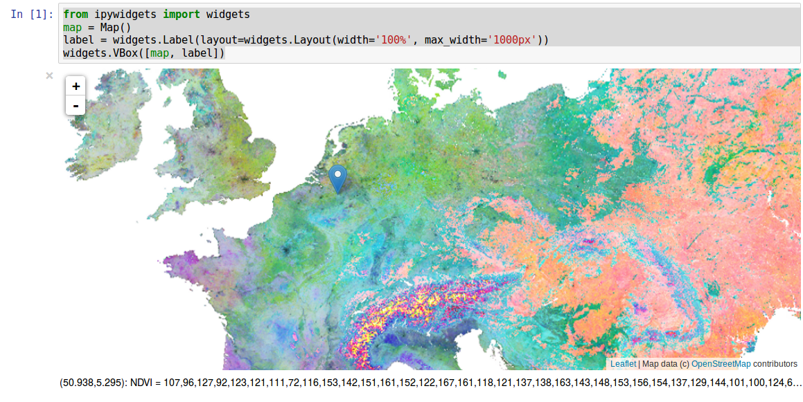
We import two modules, one for the marker and one for the plot. Each collection implements a function getAcquisitionDays(), which returns an array of all the acquisition dates of the images in the collection. We need this array for the x-axis of our plot.

We add a figure, setting the title to ‘NDVI’ and call the show function of the plot. The marker needs a call back function as an argument (OnChangedLocation), which is executed after it has been dropped on the map. We need to implement this call back function. It has the location of the marker as an argument, which is needed to identify the pixel values (identifyPoint). Notice that the first two arguments represent the position in x and y and correspond to the longitude (location[1]) and latitude (location[0]) respectively. The third argument is the EPSG code of the coordinate reference system (epsg:4326). We are not interested in the identifier “NDVI = “, which we can easily replace with an empty string:

from jeodpp.imap import Marker
from bqplot import pyplot as plt

dates = coll.getAcquisitionDays()
p = coll.process()
p.opacity(128)
map.clear()
tlayer = map.addLayer(p.toLayer())

plt.figure(1, title='NDVI', animation_duration=1000)
plt.show(display_toolbar=False)
def OnChangedLocation(event, location):
    global ndvi_values
    string_values = p.identifyPoint(location[1],location[0],4326).replace("NDVI = ","")
    ndvi_values = [int(s) for s in string_values.split(',')]
    plt.clear()
    plt.plot(dates, ndvi_values)

mark = Marker(location=map.center,opacity=0.9)
map += mark
mark.on_move(OnChangedLocation)

You can easily adapt the call back function OnChangedLocation to customize the interactive plot. As an example, we will plot a Gaussian filtered version of the NDVI time series:

coll = inter.ImageCollection("NDVI")
coll = coll.filterOnDate(2000,1,1,2005,7,31)
plt.figure(1, title='NDVI', animation_duration=1000)
plt.show(display_toolbar=False)
p = coll.process()
p.opacity(128)
tlayer = map.addLayer(p.toLayer())
mark = Marker(location=map.center,opacity=0.9)
map += mark
from scipy.signal import gaussian
from scipy.ndimage import filters
b = gaussian(21, 5)
def OnChangedLocation(event, location):
    global ndvi_values
    string_values = p.identifyPoint(location[1],location[0],4326).replace("NDVI = ","")
    ndvi_values = [int(s) for s in string_values.split(',')]
    ndvi_filtered = filters.convolve1d(ndvi_values, b/b.sum())
    plt.clear()
    plt.plot(dates, ndvi_values)
    plt.plot(dates, ndvi_filtered,colors=['red'])
mark.on_move(OnChangedLocation)

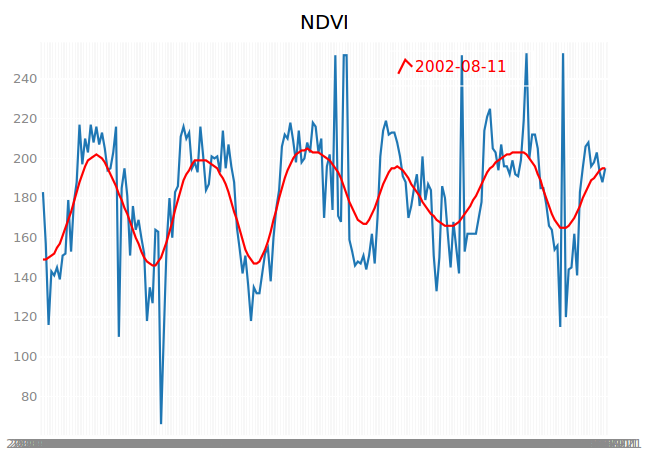
In addition, we create a label for the filtered ndvi values, showing the date of the maximum filtered NDVI. We need to add two attributes similar to the color:

• labels=[‘the label’]
• display_legend=True

The function OnChangedLocation is now:

import numpy as np
from scipy.signal import gaussian
from scipy.ndimage import filters
b = gaussian(21, 5)
def OnChangedLocation(event, location):
    global ndvi_values
    string_values = p.identifyPoint(location[1],location[0],4326).replace("NDVI = ","")
    ndvi_values = [int(s) for s in string_values.split(',')]
    ndvi_filtered = filters.convolve1d(ndvi_values, b/b.sum())
    maxIndex=np.argmax(ndvi_filtered)
    maxNdvi=ndvi_filtered[maxIndex]
    plt.clear()
    plt.plot(dates, ndvi_values)
    plt.plot(dates, ndvi_filtered,colors=['red'], display_legend=True, labels=[str(dates[maxIndex])])
mark.on_move(OnChangedLocation)